colourcats
Categorical Colour Perception in artificial networks
Abstract
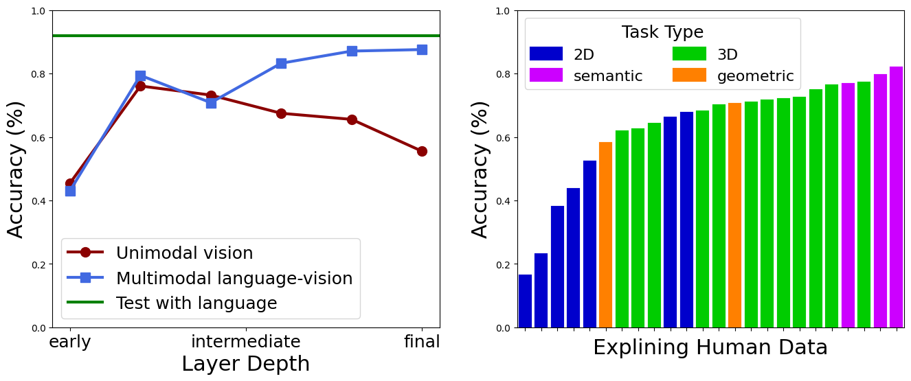
This study delves into the categorical aspects of colour perception, employing the odd-one-out paradigm on artificial neural networks. We reveal a significant alignment between human data and unimodal vision networks (e.g., ImageNet object recognition). Vision-language models (e.g., CLIP text-image matching) account for the remaining unexplained data even in non-linguistic experiments. These results suggest that categorical colour perception is a language-independent representation, albeit partly shaped by linguistic colour terms during its development. Exploring the ubiquity of colour categories in Taskonomy unimodal vision networks highlights the task-dependent nature of colour categories, predominantly in semantic and 3D tasks, with a notable absence in low-level tasks. To explain this difference, we analysed kernels’ responses before the winner-taking-all, observing that networks with mismatching colour categories align in continuous representations. Our findings quantify the dual influence of visual signals and linguistic factors in categorical colour perception, thereby formalising a harmonious reconciliation of the universal and relative debates.
Rainbow
There are no discontinuities in the electromagnetic spectrum of the light reaching us from a rainbow and yet we see hues clearly separated by colour categories.
To make this more tangible, we can simulate a rainbow and check the numerical values of its constituent hues.
Hue circle in HSV colour space
We create a list of 180 hues with constant saturation and values.
We convert the rainbow_hues from HSV colour space to RGB for visualisation purposes. We can observe that the continuous function of hues appears to be separated into different categories. This separation stems from our perceptual system otherwise the HSV colour space is only an alternative representation of the RGB space that is obtained from camera sensitivity functions.

Coloured arches
The visualisation of the hue circle does not have a spatial resolution (i.e., only one row), to better appreciate the categorical colour phenomenon, we convert the hue circle into an image of coloured arches, similar to natural rainbow.
When we illustrate coloured arches, we can clearly see colour categories such as (from bottom to top):
- pink
- purple
- blue
- cyan
- green
- yellow
- orange
- red
Although to different observers the actual colour names and the number of distinct colour categories might differ, but the principle remains the same, everyone sees the continuous function in discrete categories.

RGB prediction
We can pass this rainbow image to a computational model and check its categorisation. The simplest model is the Euclidean distance towards focal colour categories. We consider two types of focal colours:
- Uniformly selected within the rainbow image.
- Focal colour categories from human data.
We can observe that this model created bands of equal width when the focal colours are selected uniformly. This is rather trivial. There is no categorical effect in a continuous space. Nevertheless, this reemphasises that any categorical colours we perceive in the rainbow image are purely driven by our visual system.
In the second scenario, where focal colours are selected from human data, we observe that the RGB prediction is not uniform but still does not resemble our perception. For instance, The blue and orange categories are disproportionally large suggesting the computation behind our categorical colour perception is not a simple smallest distance in the input space and some nonlinearity is necessary.

Open questions
This is a fascinating phenomenon that raises the following questions:
- Why do we perceive a continuous function in different categories?
- Are these categories shared among everyone or are there significant individual differences?
- Is the categorical colour perception because of linguistic terms we assign to colours and/or this is purely driven by our visual system?
In this project, we used deep neural networks as a framework to study some aspects of categorical colour perception:
- We compare multimodal vision-language to unimodal vision deep neural networks to investigate the role of language.
- We compare 24 networks pretrained on an identical dataset for 24 distinct tasks to investigate the role of visual tasks.
- We compare two convolutional neural networks (CNN) to vision transformers (ViT) to investigate the role of architecture.
- We compare representation at different intermediate layers to investigate whether this is low-, mid, or high-level representation.
Stimuli
In this section we describe the stimuli set we used to evaluate networks.
Munsell chips
We use 320 Munsell chips to evaluate our networks. These chips have been extensively used in the literature of categorical colour perception.

Human data
We rely on human-data for 8 chromatic colour categories (Berlin & Kay, 1969; Sturges & Whitfield, 1995).


Shapes
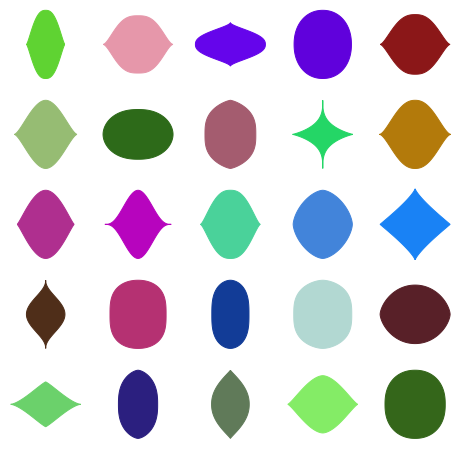
We generated 2904 shapes by systematically changing five parameters of superellipse equation:
\[\left| \frac{x}{a} \right| ^{m} + \left| \frac{y}{b} \right| ^{n} = 1\]The idea behind using a systematic geometrical shape is to investigate the interaction between object shape and colour perception. This is beyond the scope of this notebook and is part of another project.
We can plot 25 of those superellipses randomly.
Experiments
Language models: zero-shot evaluation
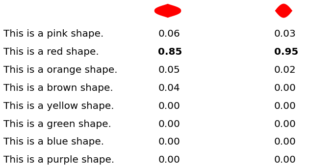
For the language models (i.e., CLIP) we can directly conduct psychophysics on the network without any intermediate step:
- For each shape, we colour it with a Munsell chip and input the network with eight phrases corresponding to eight colour terms.
- The phrase: “This is a {COLOUR-TERM} shape.” and COLOUR-TERM is one of these terms: red, orange, yellow, brown, green, blue, purple, pink.
- Network’s output is a number (the probability of the phrase matching the image). We take the phrase with the highest probability as the network’s final output.
- For each Munsell chip, we repeat this procedure for all shapes (2904), performing 23,232 trials (\(8\times 2904\)).
Let’s look at one example with simulated data. In this example, the network’s output is highest for the phrase “This is a red shape.”, therefore we take that as the network has placed this colour into the red category. The average across all 2904 shapes would be the final prediction of the network for this colour.
Vision models: odd-one-out linear classifier
It is impossible to directly ask a neural network trained on a task like object recognition about colour categories, as the neural network was specifically trained for another task. To overcome this, we trained a linear classifier to perform a 4AFC colour discrimination task and at test time evaluate whether this discrimination is categorical. That is to say, the framework to evaluate the categorical colour perception in vision models consists of two steps:
- A network is trained on an arbitrary visual task (e.g., object recognition). We refer to such a network as a pretrained network.
- Features extracted from the frozen pretrained network are input to a linear classifier trained for the colour discrimination 4AFC task. We refer to the trained linear classifier as a colour-discriminator.
Training colour-discriminator
The figure below shows the schematics of our training process.

The process of extracting features (also known as, readouts) from a pretrained network can occur at any depth of a network. We extract features from six distinct layers from the early to final layer:
- Common to all architectures:
fcfor ImageNet (classification layer) orencoderfor Taskonomy (the final encoding layer) and CLIP (the final vision layer). - In the case of
ResNet50architecture, from 5 intermediate areas (a collection of residual blocks). - In the case of
ViT-B32from blocks[1, 4, 7, 10, 11].
Train images
During the training, the linear classifier is input with four images:
- Three of those are identical.
- One odd image that only differs in colour.
The colour difference between common-odd images is drawn from a random uniform distribution ensuring no colour bias is introduced in the colour discriminator training.
The background colour is always achromatic whose luminance is drawn from a random uniform distribution

Testing paradigm
At test time, for each Munsell chip, we evaluate against all sets of focal colour pairs. For instance, for the munsell_chips[3][2], we input the network with the following four colours:
- The first and last being one focal colour (in this example pink and red categories).
- The two middle images are identical to the colour of the test chip.
We interpret the results:
- If the network outputs the pink image as odd, we conclude that the network has put the test chip into the red category.
- If the network outputs the red image as odd, we conclude that the network has put the test chip in the pink category.
We also test the network by swapping the first and last images to ensure the results are not biased towards a certain index.

For the same test chip, we repeat this procedure for all 28 combinations of pairs of focal colours:

We assign the colour that wins the most trials across all tests/shapes as the colour of the test chip.
Pretrained networks
Architectures:
- Vision Transformers (ViT) – ViT-B32
- Convolutional Neural Networks (CNN) – ResNet50
Pretrained task:
- CLIP: multimodal text-image matching
- ImageNet: unimodal object classification
- Taskonomy: 24 unimodal tasks (e.g., scene segmentation, object recognition, edge detection, denoising, etc.).
Inetrmediate layers: six distinct layers corresponding to low-, mid- and high-level visual representation.
Results
To better understand the data crunch from raw data to plotted figures, we look at one example.
Explaining with one example
We will look at the results of Block-10 of the ViT-B32 architecture (i.e., the image encoder of CLIP). The directory name bg128_i0 means the linear classifier (colour discriminator) has been trained with images of grey background (\(R=G=B=127\)).
The results are loaded into an array of shape (320, 8, 8): essentially the 320 confusion matrices of size \(8 \times 8\).
One Test chip
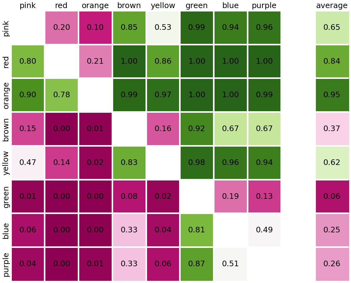
We can simply print the confusion matrix for one particular Munsell chip. We do that for chip at index 122 which corresponds to the test colour we visualised when explaining the testing paradigm:
- Each cell is the percentage of time a focal colour was selected as the odd element (i.e., lost the categorical battle to another focal colour).
- The diagonal of the matrix is 0.
- Higher values indicate strong categorical representation (e.g., orange versus all other colours). A value close to 0.50 indicates a chance level and no categorical representation.
- The confusion matrix cannot be reduced to the (upper/lower) triangle. The sum of \(C + C^T \leq 1\), where \(C\) and \(C^T\) denote the confusion matrix and its transpose. Their sum is not guaranteed to equal 1, as the selected odd index by the network can also be the identical test chip. Small numbers for \(C + C^T\) indicate the network’s representation is not categorical. Overall, it can be observed that the \(C + C^T\) is quite close to 1.
We compute the average winning rate of each focal colour and the highest value is selected as the colour of the test chip.:
- In this example orange wins against other focal colours \(95\%\) of the time.
- Note that the average column is not a true probability distribution, the sum is not equal to 1.
- A value of 0.50 indicates no categorical representation.
All chips
We compute the colour of each Munsell chip following the procedure above. We can plot this in the same format as the original Munsell image.
The plotted figure can be interpreted as follows:
- Those cells with a white colour do not have ground truth, therefore excluded.
- Other cells have taken a focal colour according to the network prediction.

We can compute the accuracy with respect to the ground truth. In this example, the network predicts human data \(83\%\) of time.
We plot x on top of the cells where the network’s prediction mismatch the human data:

Baseline – RGB Model
To put the obtained results with networks into perspective we compare them to the “RGB Model” that assigns the closest colour category (smallest Euclidean distance) to a Munsell chip:
- Eight focal colours are selected by taking the average of all Munsell chips in the Berlin & Kay (1969) and Sturges & Whitfield (1995) Ground Truth.
- For each Munsell chip, we compute the Euclidean distance to eight focal colours.
- The focal colour with the smallest Euclidean distance is selected as the colour category of that test chip.
In simple words, if the test chip is physically closest in the space to the pink category, its colour category will be pink.
One might argue that step 0 is not an accurate estimation of focal colours as the centre of mass does not necessarily determine the focal colour. Our rationale behind this baseline:
- The RGB Model categorises colours uniformly based on proximity.
- Essentially, in any colour space there is an inherent categorical effect of uniform discretisation.
- Therefore, any categorical effect we observe in the network is significant if it surpasses the RGB Model.
We computed the physical proximity in several colour spaces, including:
- DKL
- CIE L*a*b*
- RGB
- LMS
- HSV
- YPbPr
We have taken RGB as the baseline because of two reasons:
- The pattern of results across colour spaces is very similar.
- The input colour space to networks is RGB (i.e., the pretrained datasets are in RGB). Therefore we can analyse how much the colour categories alter from the input representation to the network’s internal representation.
Below, we have visualised the prediction from six different colour spaces. We can observe that although simple Euclidean distance in colour spaces can predict the human data to a certain extent, the error rate remains high (about 30%).


The role of language
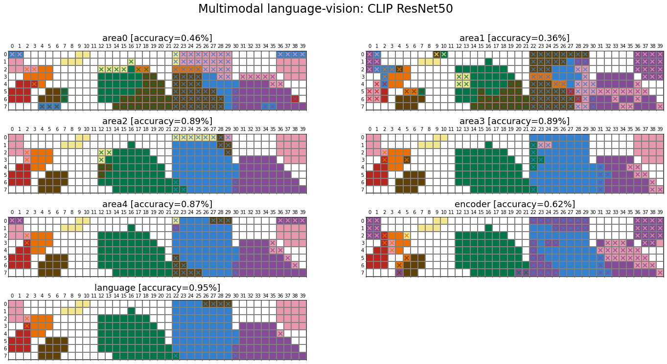
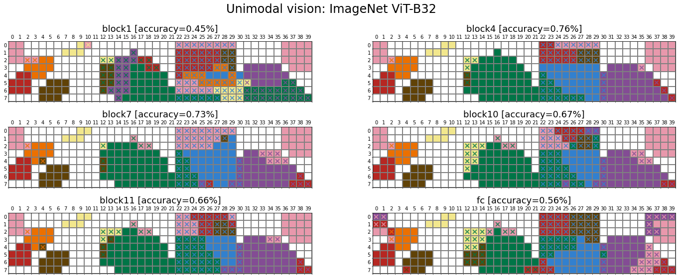
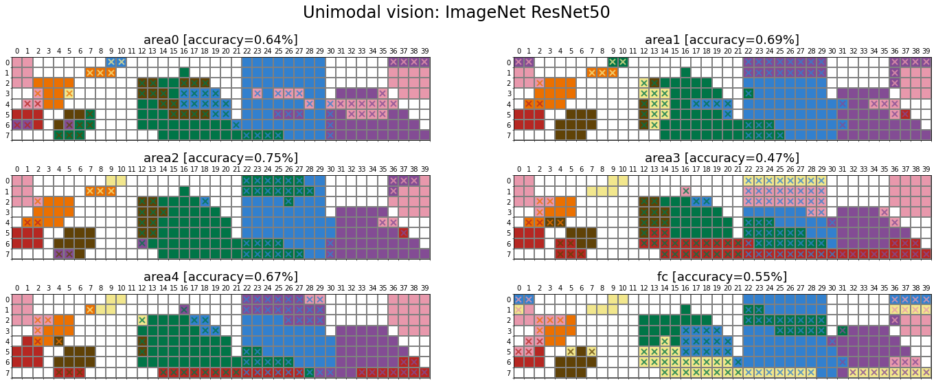
To assess the role of language on categorical colour perception, we compare the results of four networks pretrained obtained from combination of two architectures:
- Vision Transformer (ViT) – ViT-B32
- Convolutional Neural Network (CNN) – ResNet50
trained on two different tasks:
- CLIP (Multimodal language-vision)
- ImageNet (Unimodal vision).
For each of these networks, we have trained several instances to ensure the reported results are robust. Given the high degree of similarity across instances, below we visualise the results for instance 1.
CLIP - ViT-B32

CLIP - ResNet50
ImageNet - ViT-B32
ImageNet - ResNet50
Multimodal language-vision vs. Unimodal vision

The role of visual task
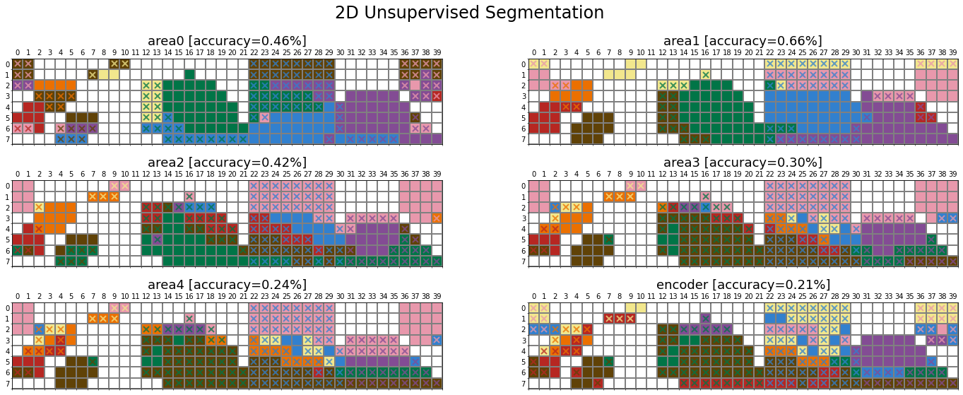
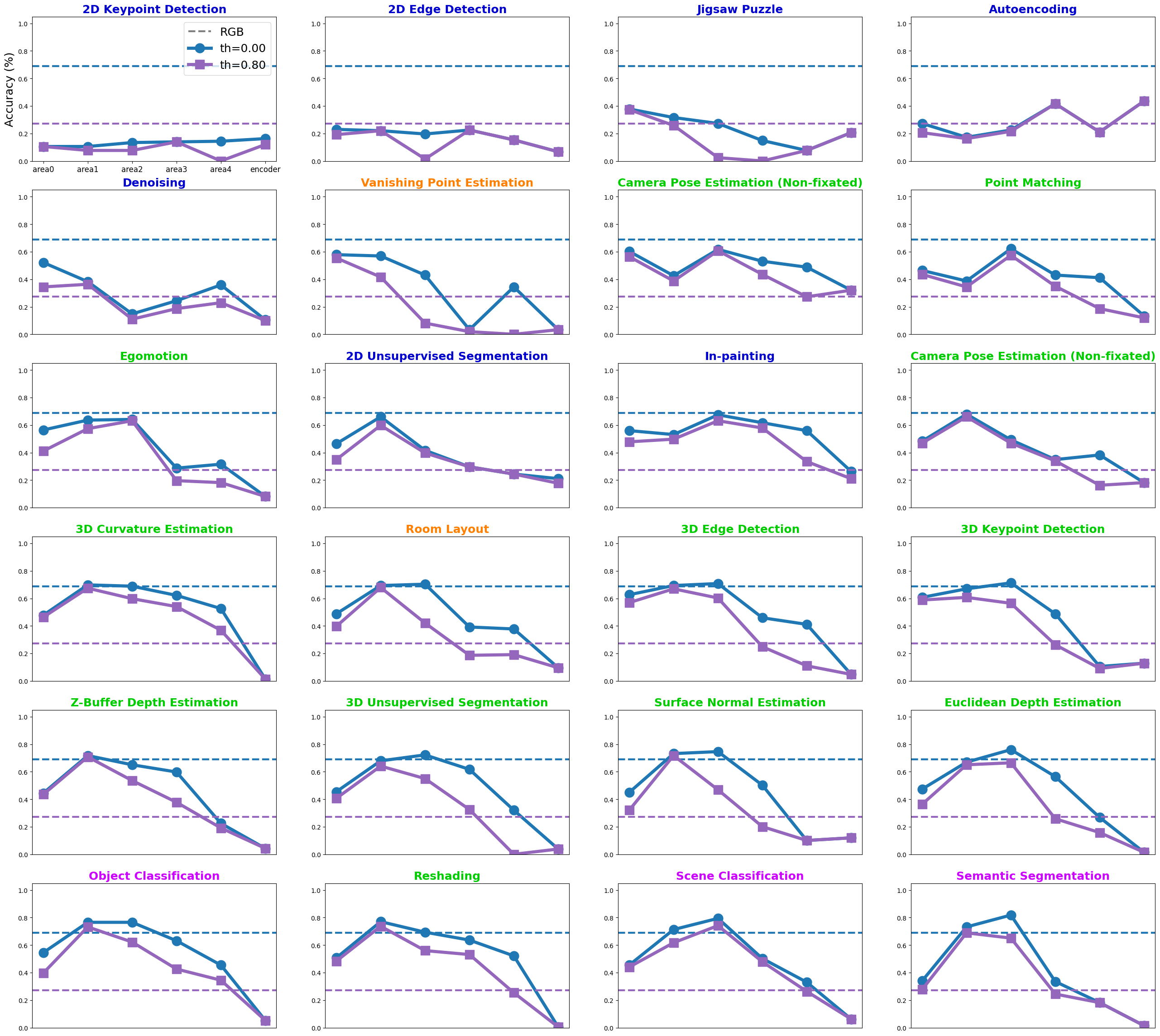
In this section, we examine how the network’s task shapes its colour categories using the Taskonomy dataset, which contains about four million images (mainly indoor scenes from 2265 different buildings) and their corresponding labels for 25 computer vision tasks. The dataset also provides pretrained networks with an encoder-decoder architecture for all visual tasks. The encoder is the same across all pretrained networks (i.e., ResNet50), which maps the input image (\(224 \times 224\)) into a latent representation of size 1568 (\(14 \times 14 \times 8\)). The decoder design varies according to the dimensionality of the task output. The encoder offers a unique opportunity to study the role of visual tasks on the representation a network learns, given its architecture is identical across tasks and has been trained on the same set of images. Similar to ImageNet pretrained networks, we trained a linear classifier on top of the encoder’s extracted features from each Taskonomy pretrained network.
Munsell prediction

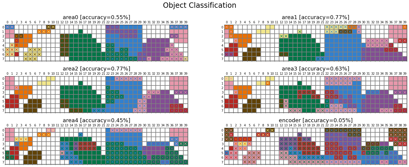
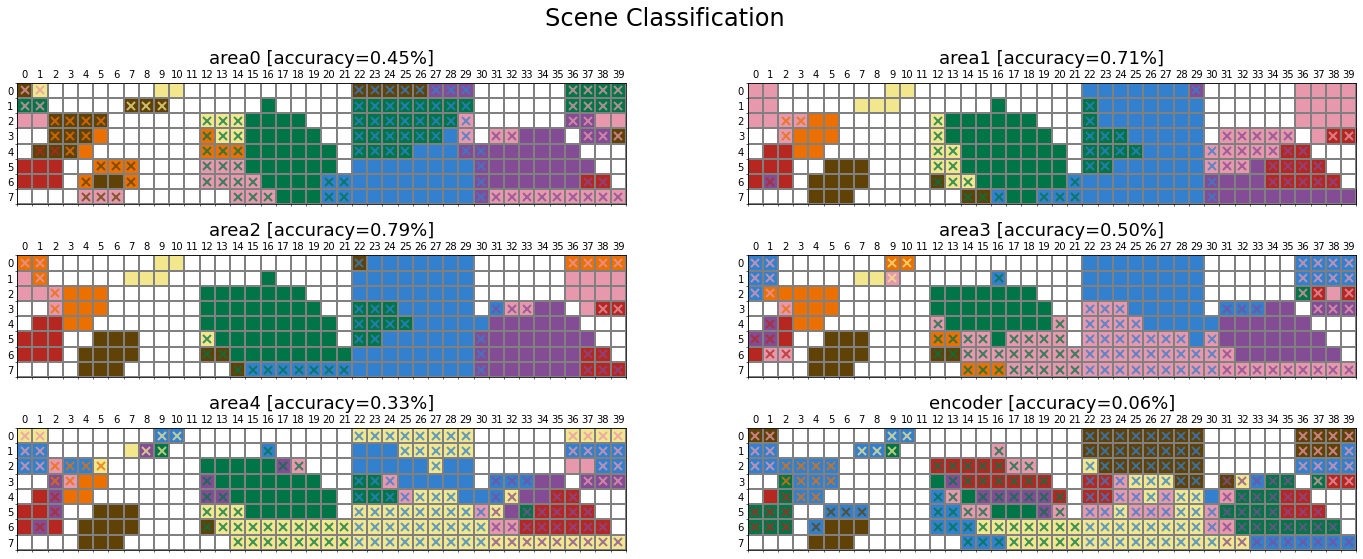


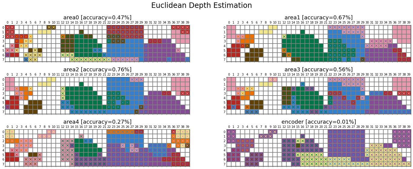
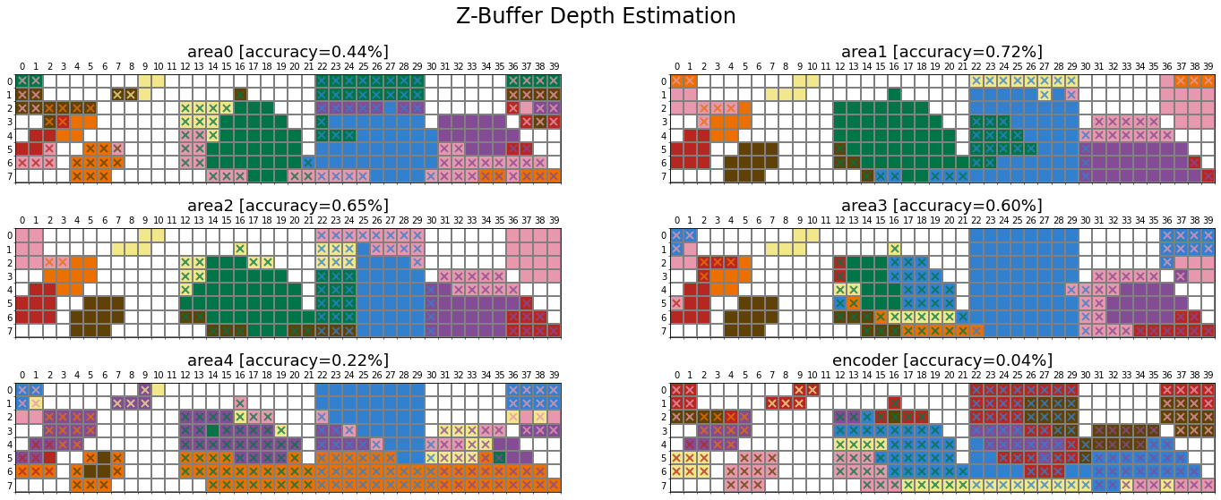
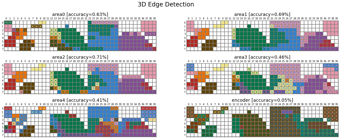
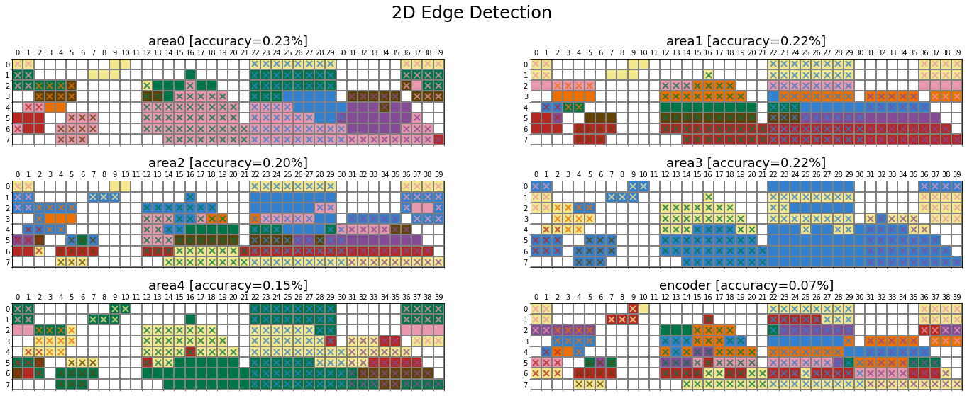
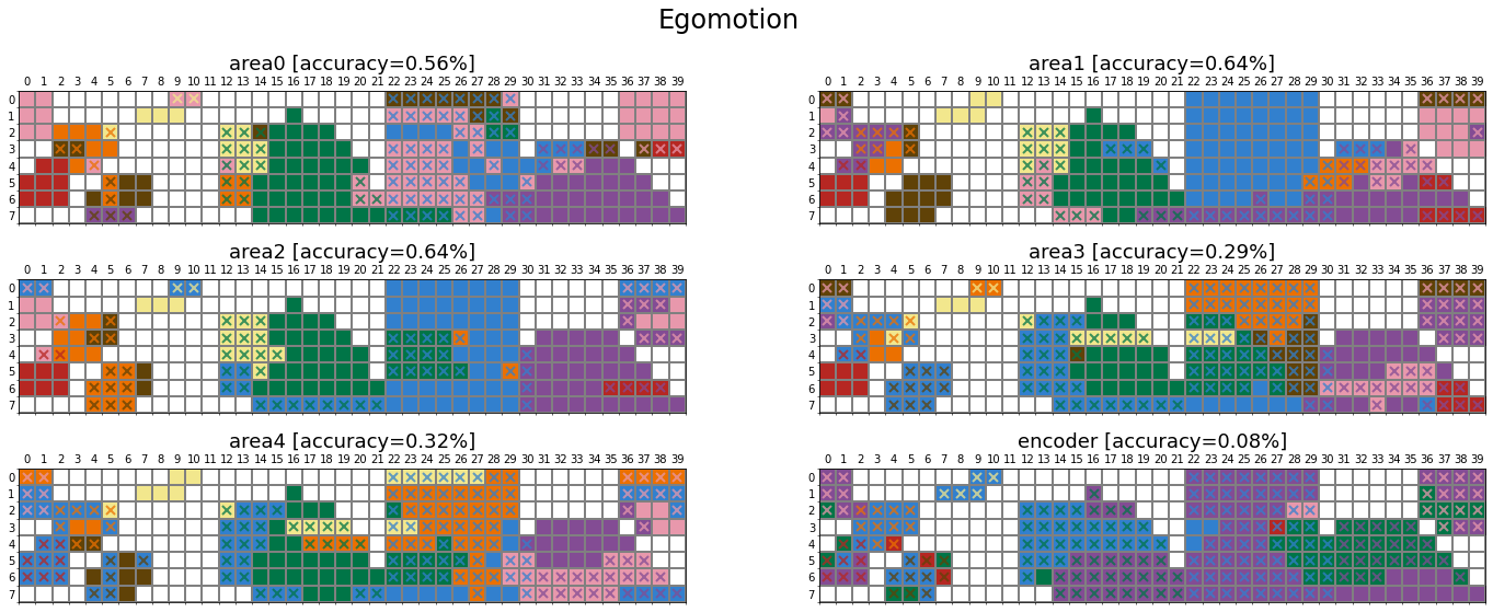
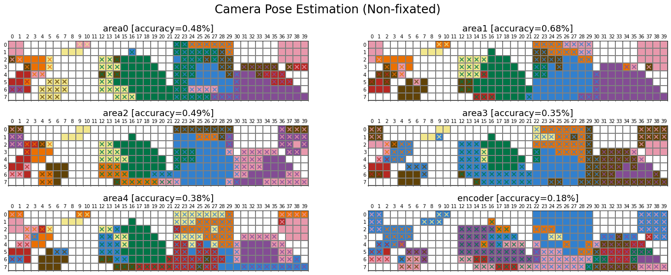
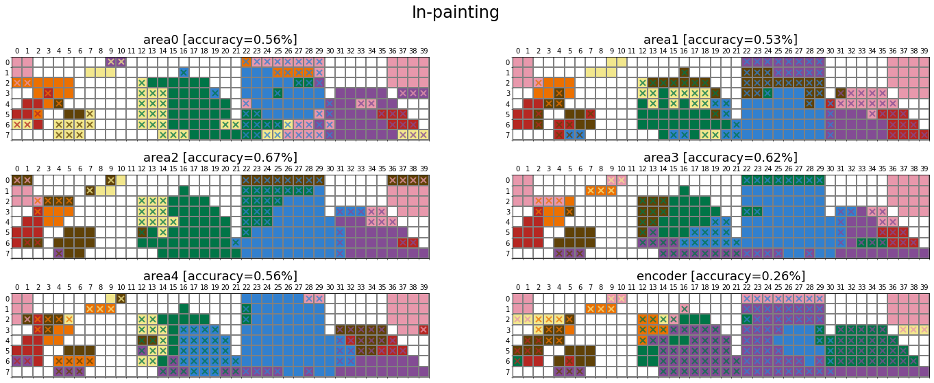
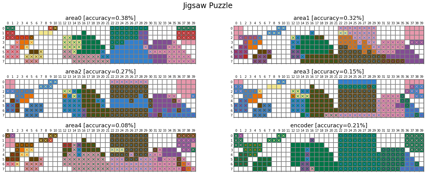
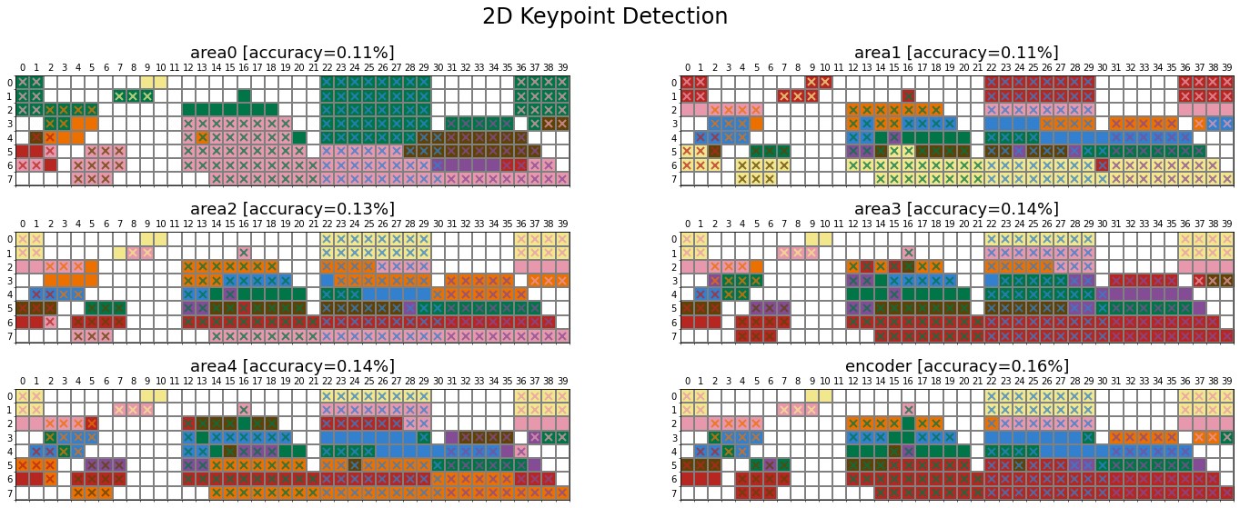
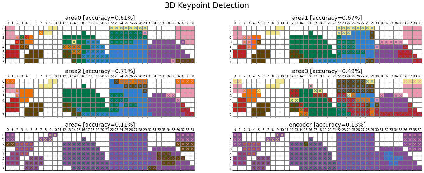

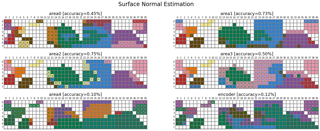
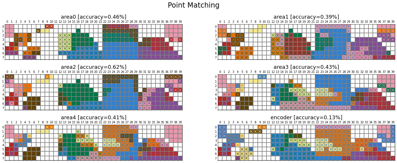

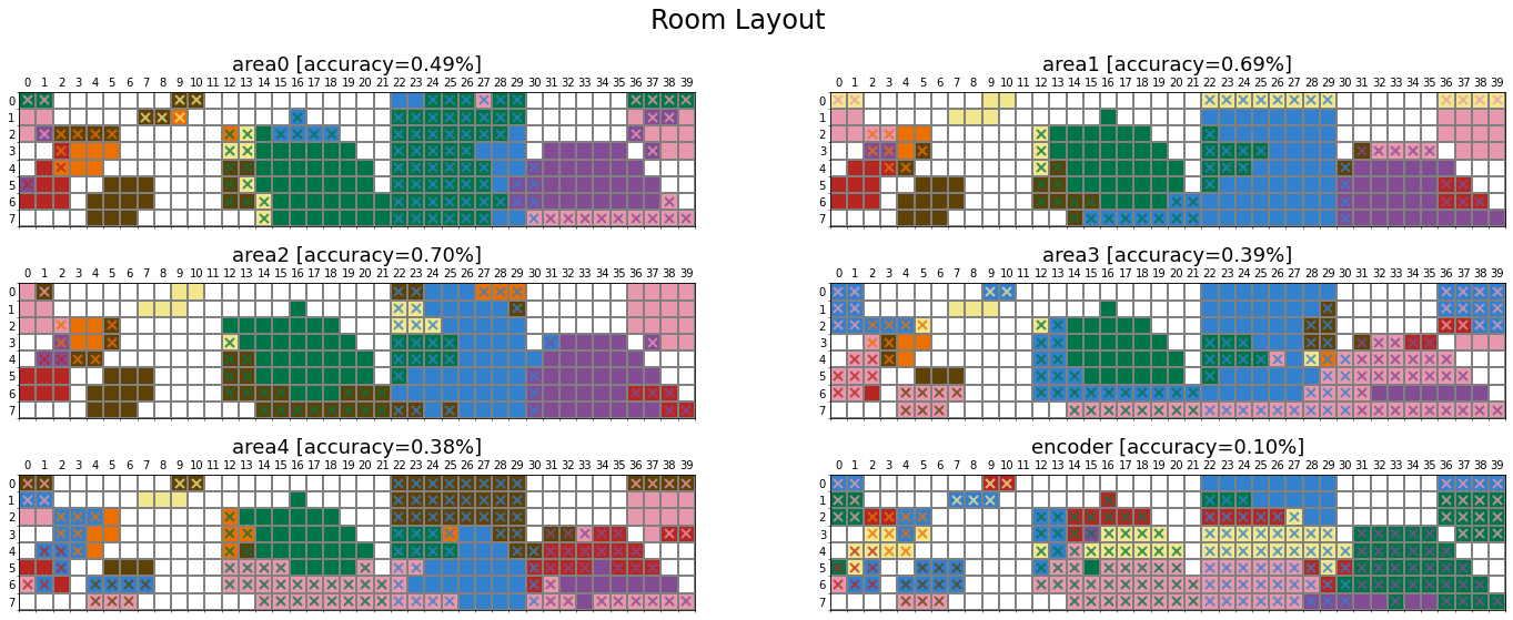
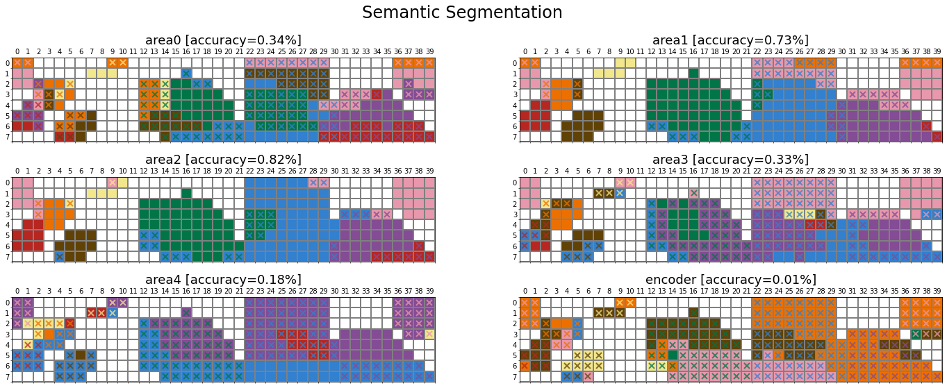
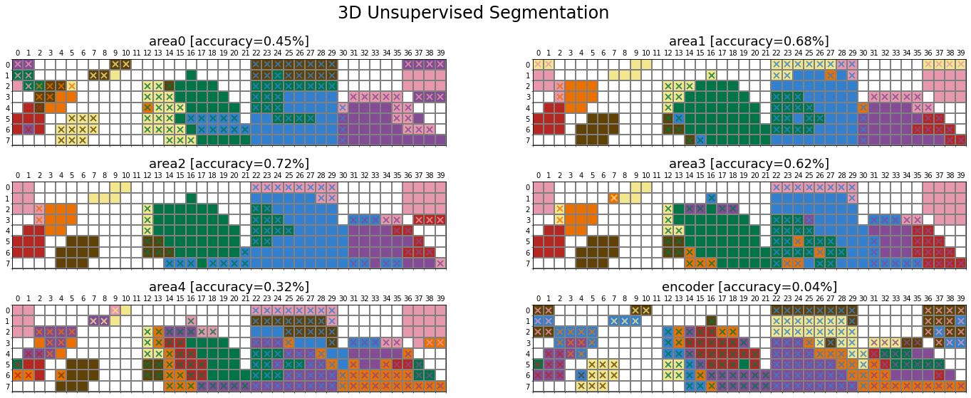

Comparison across tasks
Individual colour categories
We can compute the accuracy for each of the colour categories separately to analyse whether certain categories systematically obtain higher accuracy in comparison to the average. The figure below shows the individual colour categories averaged across all twenty-four tasks.

Internal representation
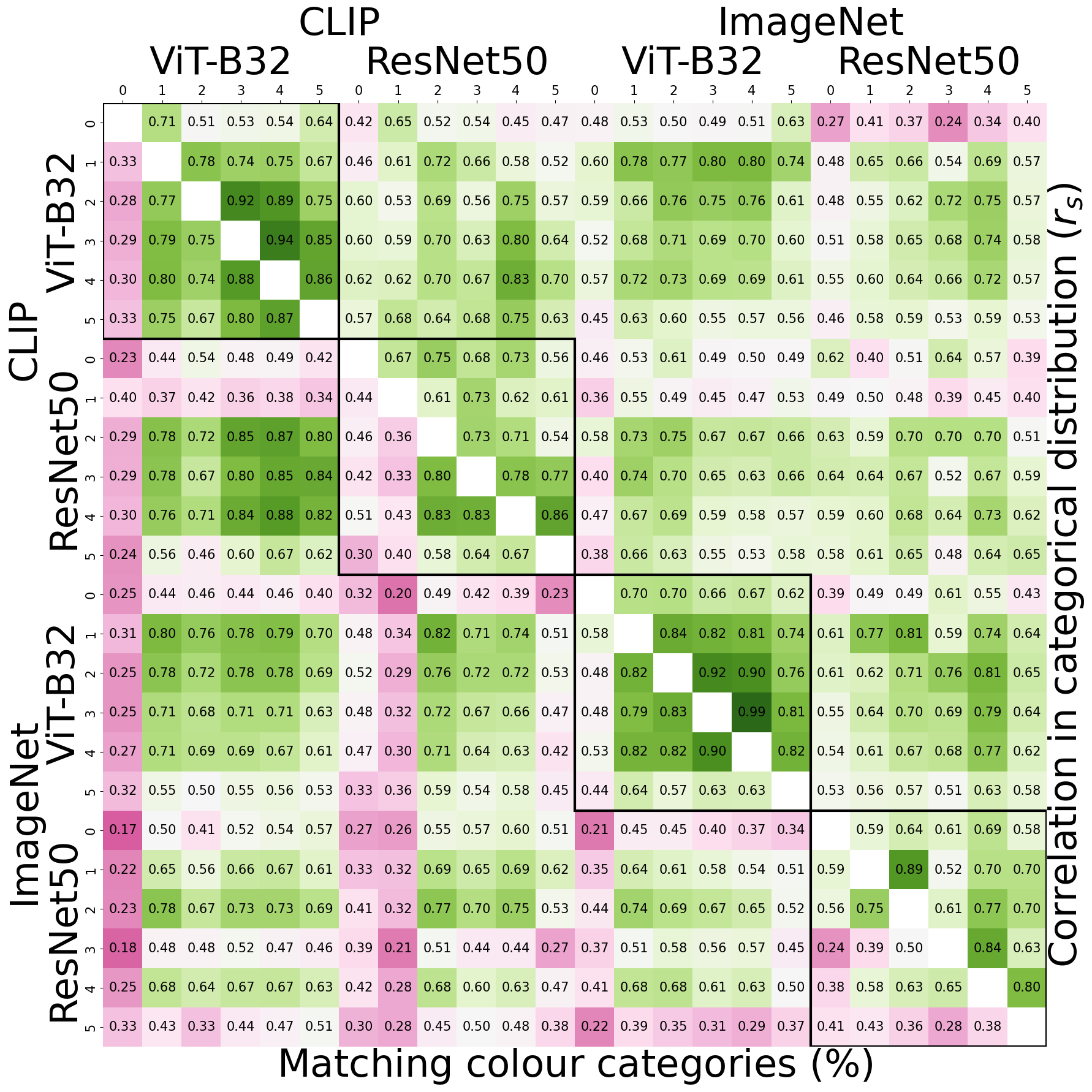
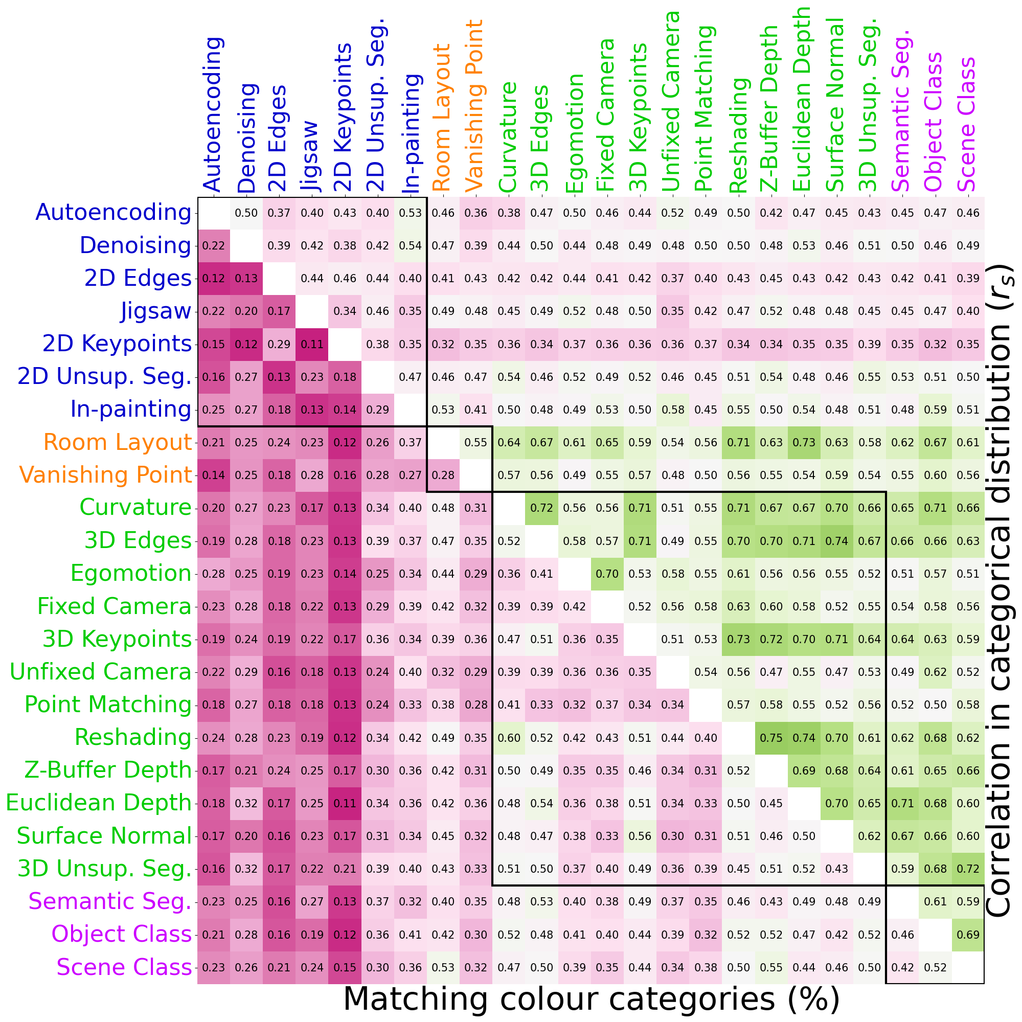
The comparison of networks/layers to human data has revealed a distinct division. Some networks/layers closely approximate human colour categories, while others fail to align with them. This raises the question of whether there is a fundamental difference in how these two groups of layers/networks represent colours. It is important to note that networks’ colour categories are determined through a winner-take-all operation on an eight-class distribution. This is essentially a discrete procedure where one colour wins the category while the rest are silenced. However, before the discretisation stage, the underlying representation is a continuous distribution of the winning ratio among pairs of colour categories, which is a matrix of size \(8 \times 8\). To compare the internal representations of colour categories in networks/layers, we calculated the average Spearman correlation coefficients on this eight-class confusion matrix for each Munsell chip.
CLIP - ImageNet
The continuous representation (upper triangle) exhibits better agreement across networks/layers compared to the discrete categories (lower triangle). The average correlation in categorical distributions (continuous) across all layers of CLIP/ImageNet ViT-B32/ResNet50 networks is \(0.63 \pm 0.12\). In contrast, the percentage of matching colour categories (discrete) shows both a lower average and higher standard deviation (\(0.54 \pm 0.18\)), indicating that the underlying continuous representations are significantly more similar than the discrete colour categories. This heightened correlation in the underlying continuous representation is particularly evident within the layers of a single network (depicted by dark-bordered squares; \(r_s=0.72 \pm 0.04\)), and it is notably pronounced in ViT networks.
Taskonomy
The presented comparisons between networks are averaged over layerwise values (i.e., six layers). The first notable observation is the low ratio of matching colour categories across all 24 Taskonomy networks (purple cells in the lower triangle). This observation is not surprising, given the substantial variation in accuracy when explaining human data across different tasks. A second noteworthy pattern is the moderate green cells in the upper triangle, indicating a decent correlation (\(r_s=0.65\)) in the categorical distribution of most visual tasks, except the networks trained on 2D tasks (blue labels). This strongly suggests that although the winner colour categories for these networks are notably different, the underlying representation is not significantly dissimilar.
Rainbow qualitative prediction
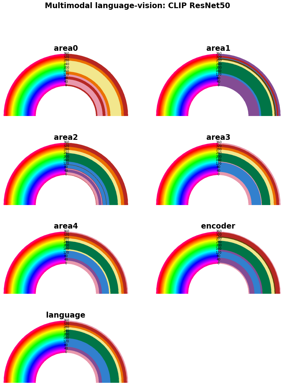
So far we have looked at the network’s prediction of Munsell chips and analysed them quantitatively. We can now qualitatively look at the network’s prediction of the rainbow image. Overall, we can observe that the networks’ prediction, at deeper layers, captures well our categorical perception. The language prediction particularly stands out. The only difference between the network’s prediction and my subjective colour perception is the colour of cyan. But of course, the network was never prompted with this colour term.

Additional colour terms
We tested the language models with an additional colour term cyan to check whether it could perfectly predict our perception of the rainbow. The results are presented in the figure below. We can see that both CLIP models, irrespective of the architecture of their vision encoder predict the cyan rings in between blue and green categories.

Discussion
- Unimodal vision models explain 85% of human data.
- The remaining 15% is explained by multimodal vision-language models.
- Categorical colour perception is a free-from-language representation, although its development is influenced by linguistic terms.
