Abstract

Our colour perception diverges from objective photometric measurements in several aspects. One prominent example is the colour difference between two surfaces. Despite numerous attempts, no colour spaces are genuinely perceptually uniform, i.e., a perfect match between the spatial distance of two colours and the perceived colour difference. Here, we put forward a novel approach by utilising deep neural networks (DNNs) to tackle this challenge. We train a linear classifier on top of frozen pretrained networks to perform a colour discrimination odd-one-out task. Next, we measure the networks’ sensitivity threshold for several RGB points in multiple directions. The pattern of networks’ discrimination thresholds highly resembles human sensitivity, e.g., higher sensitivity to hue than chroma. Next, we train a shallow neural network to transfer the RGB space into a new space with a homogenous Euclidean distance for all measured sensitivity thresholds. Our evaluation of this deep colour space on several human data suggests this framework can potentially lead us to find a perceptually uniform colour space.

Colour spaces

A colour space is an arbitrary definition of colours’ organisation in space. Since human colour vision starts with three types of cone photoreceptors, most (if not all) colour spaces are defined in three-dimensional space. In theory, an infinite number of colour spaces could be formulated, and indeed several exist in the literature and industry. RGB is the standard in digital photography, and consequently widely used in machine vision.

RGB

RGB represents colours by three additive primaries in a cubic shape. The corresponding colours for all eight corners of the cube are illustrated below. In the presence of only one primary, we obtain red, green and blue colours. A combination of two of the primaries results in yellow, purple and cyan colours. Finally, the presence and absence of all primaries produce white and black, respectively.

We uniformly sample one thousand points from this space and use it to visually compare different colour spaces. We plot such data in four inserts:

• The leftmost insert is a 3D illustration of sampled points.
• The other three inserts show the same points in 2D planes.

In the visualisation above, several points lie exacly on top of each other, therefore, it might be more informative to inspect plane slices of the space without any points overlapping:

• Coronal: where R is constant.
• Sagittal: where G is constant.
• Transverse: where B is constant.

Coronal plane

Sagittal plane

Transverse plane

Other colour spaces

Let’s look at a few other popular colour spaces to obtain a different view of how colour can be structured in the space. We convert the entire RGB gamut (all the one-thousand RGB points) into different colour spaces.

DKL

The DKL colour space (Derrington-Krauskopf-Lennie) models the opponent responses of rhesus monkeys in the early visual system:

• It transforms the RGB by a \(3 \times 3\) matrix (i.e., rotation, shearing, scaling and reflection).
• The axes approximately correspond to luminance, red-cyan, and yellow-blue channels.

YCC

The YCC (also known as \(YC_oC_g\) or \(YC_1C_2\)) decorrelates the RGB channels by a fast computation:

• It uses a \(3 \times 3\) transformation matrix whose coefficients are simple binary fractions.
• The axes approximately correspond to luminance, orange-blue, and green-violet channels.

HSV

The HSV colour space (hue, saturation, and value) is a cylindrical representation of the RGB cube designed by computer graphics:

• The white and black points are set as the origins of the top and bottom bases of the cylinder.
• The transformation forces the RGBCMY into a plane to obtain a circular hue.

CIE Lab

The CIE Lab colour space (luminance, red-green and yellow-blue axes) intends to be perceptually uniform:

• The transformation consists of going into the XYZ space by linearising relative to a white point.
• The luminance channel is effectively a power curve with an exponent of \(\approx 0.43\).

Colour difference

A colour space is perceptually uniform if the spatial distances between two colours in that space perfectly match the colour difference humans perceive.

Human-data

Several studies have measured colour discrimination threshold and colour differences of human visual system. We rely on the following data:

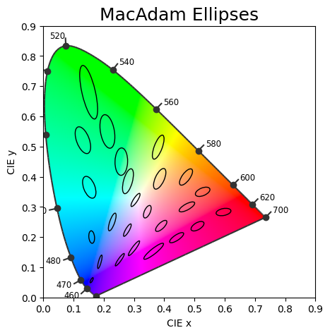
1. MacAdam ellipses (1942)
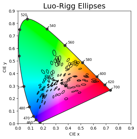
2. Luo-Rigg ellipses (1986)
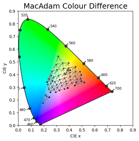
3. MacAdam colour difference (1974)

MacAdam Ellipses

The idea behind MacAdam ellipses is that within each ellipse, colours are indiscriminate to human eyes. `

Luo-Rigg Ellipses

The idea behind Luo-Rigg ellipses is similar to MacAdam ellipses. However, contrary to the MacAdam Luo-Rigg ellipses have different luminance \(Y\) values.

MacAdam 1974

The lines from each point towards different direction indicates the relative magnitudes of colour difference.

Quantifying goodness

1. Colour discrimination data:

   To quantify uniformity of a colour space, we rely on standard deviation (\(\sigma\)) among measured sensitivity thresholds. The figure below depicts the Euclidean distance in RGB colour space for a set of measured points. In a perceptually uniform colour space, all these distances should have an identical length, therefore:

   • A small standard deviation indicates greater uniformity.
   • A large standard deviation indicates nonuniformity.

   It is important to note that the absolute distance that determines the sensitivity does not determine the uniformity.

   Naturally, the standard deviation depends on the absolute values. Therefore, when comparing different colour spaces, we ensure the space is normalised to the range from 0 to 1.

2. Colour difference data

   We use the correlation coefficient (\(r\)) to quantify how much a colour space predicts human colour difference data such as MacAdam 1974.

Metrics

To better explain the problem, we have sampled three orthogonal planes from the RGB space. Next, we will draw lines between all pairs of neighbouring points according to difference colour difference metrics. The line’s length indicates the distance between the points:

• Longer lines denote bigger colour differences.
• Shorter lines denote smaller colour differences.

Euclidean distance

In the figure below, we have used the Euclidean distance in RGB colour space as our colour difference metric. Naturally, since sampled points were drawn from a uniform distribution in RGB, the distance between all neighbouring points is identical as depicted by lines. However, we know that RGB does not capture the perceive colour difference.

\(\Delta E2000\)

CIELab colour space was designed to capture the perceived colour difference better. Since the Euclidean distance in CIELab did not adequately resolve the perceptual uniformity issue, the CIE refined their definition and introduced \(\Delta E2000\) which is widely used as the colour difference metric. The figure below depicts the \(\Delta E2000\) distance between neighbouring points.

Predicting human data

The figure below compares the prediction power of different colour metrics. The

• Euclidean distance across different colour spaces (RGB, YCC, DKL, Lab) results in a similar prediction.
• \(\Delta E2000\) performs better than any of the Euclidean distances.

Although \(\Delta E2000\) is one of the best available colour difference metrics, it has the following limitations:

1. It does not fully match the human perceptual distances.
2. It is not a space but a non-Euclidean distance.

Colour discrimination in deep networks

It is impossible to directly ask a neural network trained on a task like object recognition about colour discrimination, as the neural network was specifically trained for another task. To overcome this, we trained a linear classifier to perform a 4AFC colour discrimination task, and at test time systematically measured the network’s sensitivity at different points. That is to say, the framework to evaluate the colour discrimination thresholds in deep networks consists of two steps:

1. A network is trained on an arbitrary visual task (e.g., object recognition). We refer to such a network as a pretrained network.
2. Features extracted from the frozen pretrained network are input to a linear classifier trained for the colour discrimination 4AFC task. We refer to the trained linear classifier as a colour-discriminator.

Training colour discriminator

The figure below shows the schematics of our training process.

The process of extracting features (also known as, readouts) from a pretrained network can occur at any depth of a network. We extract features from six distinct layers from the early to final layer:

• Common to all architectures: fc for ImageNet (classification layer) or encoder for Taskonomy (the final encoding layer) and CLIP (the final vision layer).
• In the case of ResNet50 architecture, from 5 intermediate areas (a collection of residual blocks).
• In the case of ViT-B32 from blocks [1, 4, 7, 10, 11].

Train images

During the training, the linear classifier is input with four images:

• Three of those are identical.
• One odd image that only differs in colour.

The colour difference between common-odd images is drawn from a random uniform distribution ensuring no colour bias is introduced in the colour discriminator training.

The background colour is always achromatic whose luminance is drawn from a random uniform distribution

Testing paradigm

To estimate networks’ colour sensitivity thresholds, we followed the standard staircase procedure to adjust the colour of the odd-one-out item until the network’s accuracy reached \(62.5 \%\). At each trial, this accuracy is computed over 2905 shapes. The figure below illustrates a real example of the staircase procedure.

Pretrained networks

Architectures:

• Vision Transformers (ViT) – ViT-B32
• Convolutional Neural Networks (CNN) – ResNet50

Pretrained task:

• CLIP: multimodal text-image matching
• ImageNet: unimodal object classification

Intermediate layers: six distinct layers corresponding to low-, mid- and high-level visual representation.

Test Points

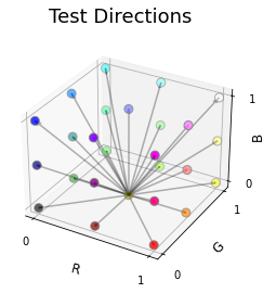
We sampled the RGB space uniformly with steps of \(0.25\). This results in 125 test points, which are illustrated in the figure below.

From each test point, we computed the sensitivity towards the outer surface of the RGB cube. An example of this is illustrated in the figure below.

Results

For each pretrained network we trained five instances of linear classifier. The results across these five instances are identical, therefore in this notebook we report the results only for one instance.

Explaining with one example

We will look at the results of Block-7 of the ViT-B32 architecture (i.e., the image encoder of CLIP). The directory name bg128_i0 means the linear classifier (colour discriminator) has been trained with images of a grey background (\(R=G=B=127\)).

Raw sensitivity thresholds

In the figure below, we have visualised the sensitivity threshold for 125 test points summing to a total of 3152 comparisons. The inserts are sorted following the standard deviation in sensitivity thresholds for the test colours. In each insert, the square marker indicates the test colour whose RGB coordinates are also written in the title. All circles correspond to the sensitivity threshold in different directions.

We can observe:

• Some of the point clouds are very small while others spread.
• If RGB were the perceptually uniform space for this layer, we would see equal-sized point clouds for all test points.
• This nonuniformity suggests more sensitivity at certain parts of the colour space is useful for the pretrained task.

Quantifying uniformity

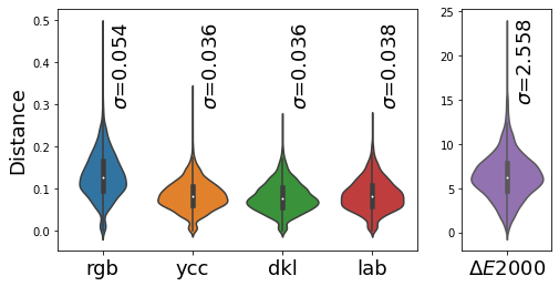
We can compute the uniformity metric (standard deviation among distances) for different colour spaces and colour difference metrics. Overall, we can see the values of \(\sigma\) are small across colour spaces:

• Smaller standard deviation in YCC and DKL colour space in comparison to RGB suggests these colour spaces are perceptually more uniform for this layer.
• \(\Delta E\) of 2.56 is slightly above JND, suggesting the network’s colour sensitivity is not far away from humans.

The role of architecture

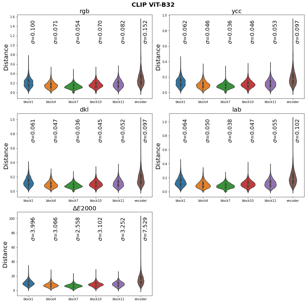
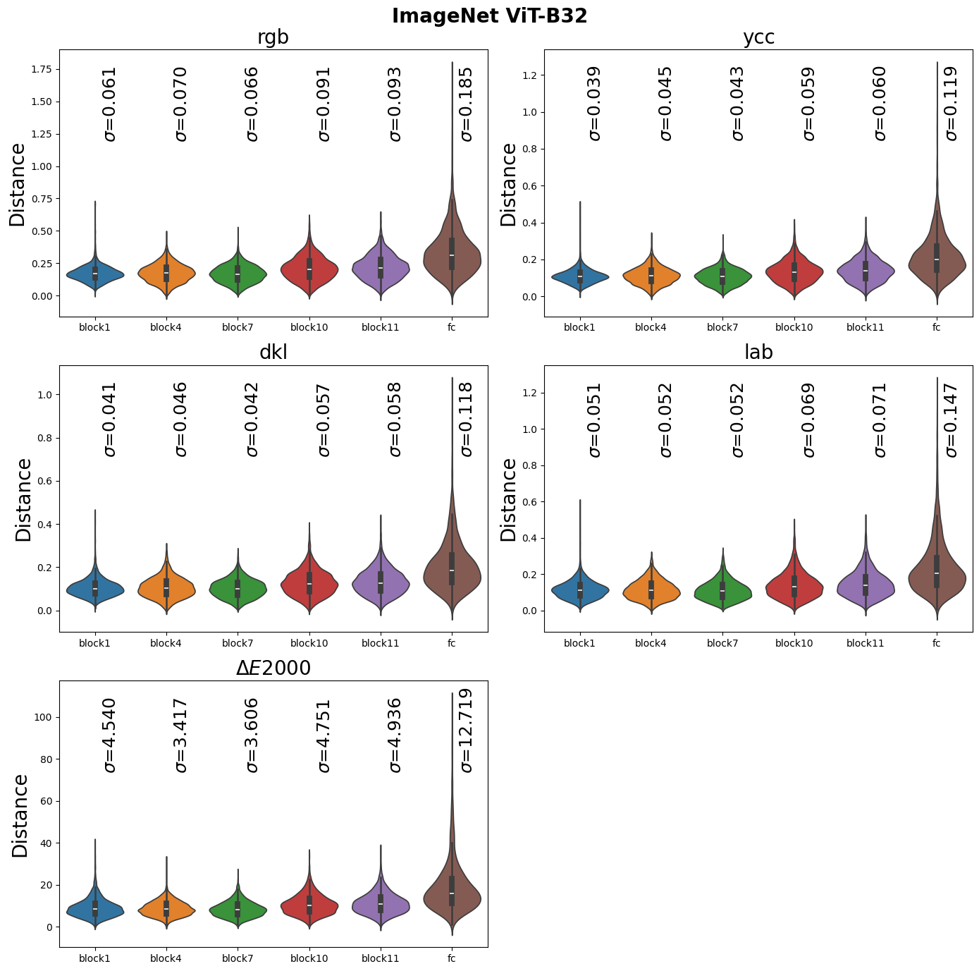
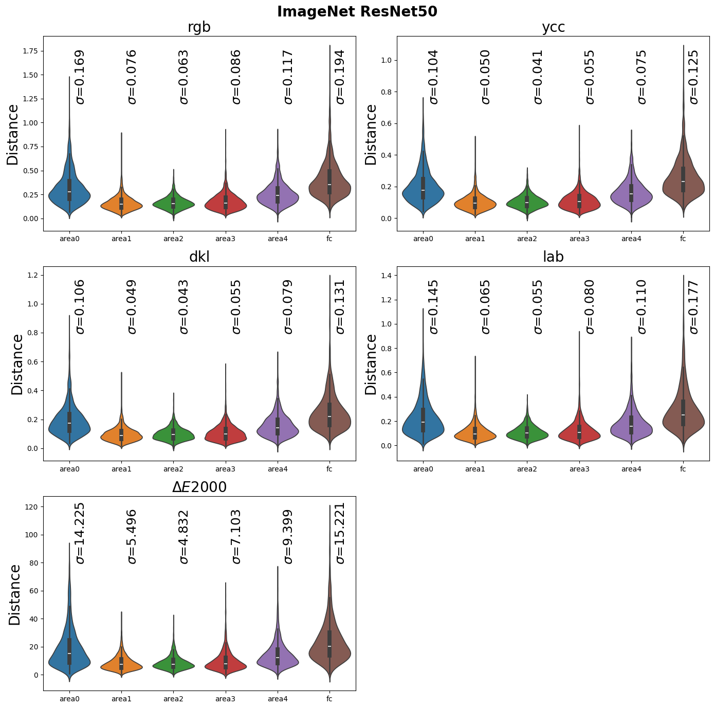
Plotting the sensitivity thresholds for all 125 test points across six readout layers results in too big of a figure. But to showcase the differences across layers (from early- to mid- and deep layers) we illustrate the sensitivity thresholds for all eight corners of the RGB cube.

CLIP - ViT-B32

CLIP - ResNet50

ImageNet - ViT-B32

ImageNet - ResNet50

Transformer vs. Convolution Networks

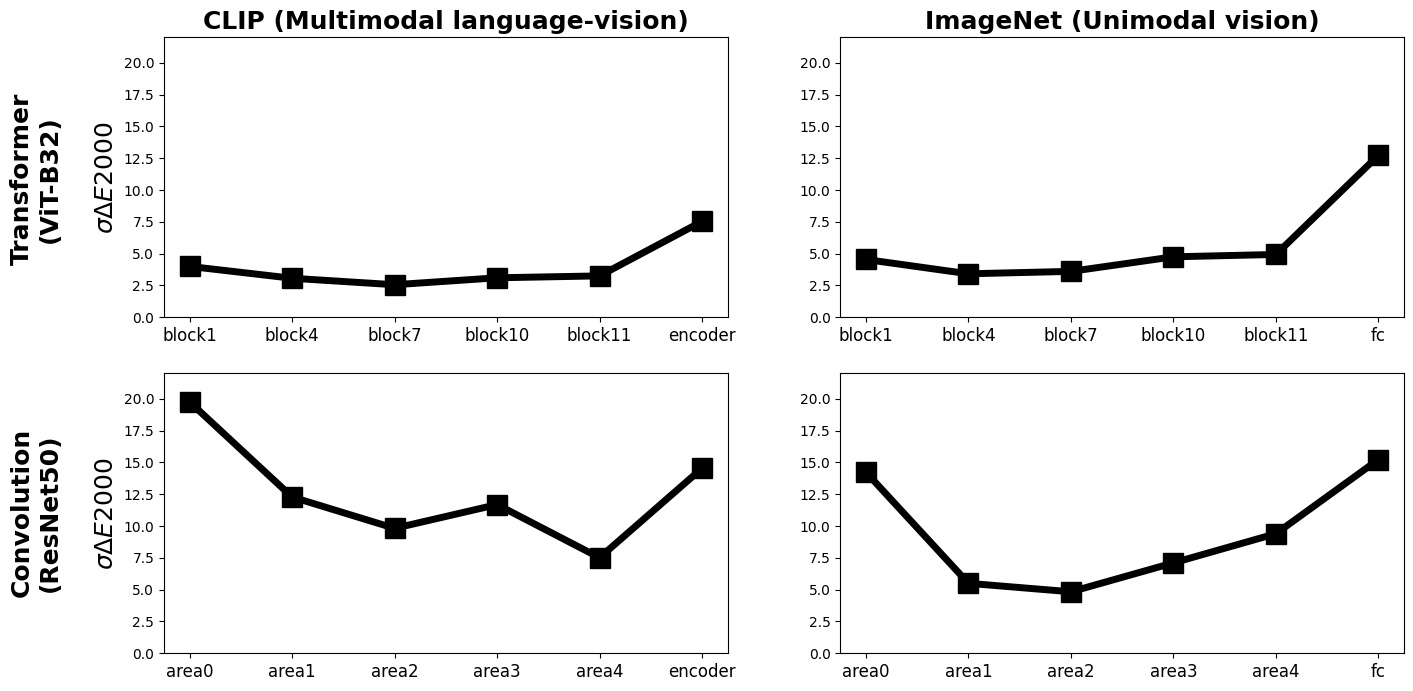
The figure below compares the colour sensitivity of networks in a confusion matrix style like across two tasks and two architectures:

• There is no significant difference between columns one and two, suggesting that language does not crucially impact the network’s colour sensitivity thresholds.
• A large difference can be observed between the first and second rows, suggesting a strong role of the network’s architecture in the network’s colour sensitivity thresholds. Vison Transformers (ViT) obtain considerably lower \(\Delta E2000\)s, which suggests they capture human sensitivity better than convolutional networks.

Optimising a uniform space

Now that we have measured a large set of sensitivity thresholds for a network/layer, we can use optimisation techniques to transform the input space (RGB, i.e., the input space of all examined pretrained networks is RGB) to a new space (we refer to it as network-space), where the standard deviation in the Euclidean distance of all measured distances equals zero (\(\sigma_{network-space}=0)\).

There are at least two good candidates to perform this optimisation:

1. Classical minimisation: defining the type of transformation (e.g., \(3 \times 3\) matrix or affine transformation, with or without exponential factor and certain nonlinearities.
2. Neural networks: deciding a neural network (i.e., set of linear and nonlinear layers) to find the optimal solution.

The benefit of the “classical minimisation” approach is that the inverse operation is given. However, it is limited to a design envisaged by us, therefore perhaps not finding the true uniform space. The benefit of the “neural networks” approach is its flexibility in finding an optimal solution. The drawback is that the inverse to RGB is not given and must be approximated.

Neural networks

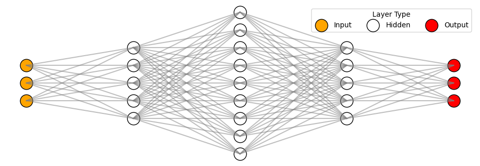
We can train a simple neural network with a few hidden (intermediate) layers to transform RGB input space to output network-space. An example of such a network is depicted in the figure below:

• This is not a schematic illustration and the number of nodes corresponds to a real scenario.
• The neural networks trained to find the uniform colour space are shallow with a few hundred parameters.
• All layers are fully-connected (also known as linear or dense layer), where all input nodes are connected to all output nodes.
• Between any two dense layers, there is a nonlinear activation function.

We can perform a hyperparameter search about:

• The number of hidden layers.
• The number of units in each layer.
• The type of nonlinearity function at each layer.

Training

We train our perceptually uniform colour space network (PucsNet) with following settings:

• 0.1 learning rate, which is reduced by one order of magnitude at every one-third of total epochs.
• 5000 epochs
• At every epoch, PucsNet transfers 3152 RGB points into the new space.
• The main term in the loss function is the uniformity metric (i.e., standard deviation among all measured distances). However, without any further constraint, the first solution the network finds is to make the data range tiny, which is not a valid solution. Therefore, we add a second term to our loss function to ensure the output range is approximately 0 to 1.

PucsNets

The optimisation explained above might end up in an infinite number of spaces all reaching the minimum loss function. Let us have a look at a few instances of PucsNets that we have trained and discuss the results.

We report the network training evolution with the following figure:

• The evolution of loss as a function of number of epochs.
• The prediction of human colour discrimination ellipses (i.e., MacAdam 1942 and Luo-Rigg 1986).
• The prediction of human colour difference (i.e., MacAdam 1974).
• Visualisation of all RGB points into the new network-space.

The instance below contains two hidden layers of each 8 units:

• The loss function although noisy steadily drops as we progress in the number of epochs. Note that the first peak at epoch 0 is because the first solution the network finds is to shrink the space range, but afterwards, it should satisfy the second constraint that brings the range of output to the range of 0 to 1.
• Network predicts human ellipses better than \(\Delta E2000\) (compare solid to dashed lines: lower values indicate more uniform space). However, it is also important to note that the prediction power of the network does not change as a function of epochs, suggesting that the initial weights make a significant impact.
• Network predicts human colour differences data equally good as \(\Delta E2000\). It is important to note that PucsNet is only trained with pretrained colour discrimination thresholds, the fact that it obtains decent results in colour difference (a similar but different paradigm) suggests the newfound space is indeed capturing other aspects of human colour vision.

The instance below contains two hidden layers of 8 and 9 units:

• Quantitatively the obtained results are very similar to the instance above.
• However, qualitatively the new space looks quite different from the instance above.

The instance below contains three hidden layers of 7, 14 and 9 units:

• Again we observe comparable quantitative results as above but with a different representation of colours.

It is important to emphasise that no human data has been used in any part of network training, therefore the fact that they predict human data equally or better than state-of-the-art \(\Delta E2000\) suggests great potential in using pretrained networks to obtain a perceptually uniform colour space. We can further explore the flexibility of training these networks to create a perceptually uniform colour space under different conditions, such as illumination and background.

Discussion

• Colour discrimination thresholds in pretrained networks highly resembles human sensitivity.
• Network architecture is influential: in comparison to convolution networks, vision transformers explain better human data.
• Artificial deep networks offer a novel framework to create a perceptually uniform colour space.